The economic architecture of the global internet relies on the strategic balancing of internet peering cost metrics against the logistical overhead of wholesale IP transit. Modern network infrastructure demands a granular understanding of how throughput and latency relate to the physical and logical interconnection points between Autonomous Systems (ASAs). The fundamental problem addressed by this manual is the volatility of egress costs: specifically, the lack of visibility into how asymmetrical traffic flows across Cisco or Juniper edge routers inflate operational expenditure. The solution involves a rigorous implementation of flow-based monitoring and BGP community tagging to calculate the true cost of a megabit. By analyzing the encapsulation overhead and the impact of the 95th percentile billing model, architects can transition from high-cost transit providers to settlement-free peering arrangements. This technical manual provides the framework for quantifying these variables within a production network stack, focusing on the intersection of physical signal-attenuation and logical routing efficiency.
Technical Specifications
| Requirement | Default Operating Range | Protocol/Standard | Impact Level (1-10) | Recommended Resources |
| :— | :— | :— | :— | :— |
| Flow Exporter | 1:1 to 1:1000 Sampling | IPFIX / NetFlow v9 | 9 | 16 vCPU / 32GB RAM |
| BGP Routing Stack | 1M+ IPv4 Prefixes | RFC 4271 (BGP-4) | 10 | 8 Core / 16GB RAM |
| API Integration | < 500ms Response | PeeringDB REST API | 5 | 1 Core / 2GB RAM |
| Interface Metric | 10G / 100G / 400G | IEEE 802.3ba/bs | 8 | SFP28/QSFP-DD |
| Telemetry Bus | 100k+ messages/sec | gNMI / gRPC | 7 | 4 Core / 8GB RAM |
The Configuration Protocol
Environment Prerequisites:
Successful deployment of a cost-analysis engine requires Ubuntu 22.04 LTS or a similar carrier-grade Linux distribution. The core routing software must be BIRD 2.x or FRRouting (FRR) to handle large-scale route tables. For physical monitoring, administrators must have access to SNMP v3 credentials and have configured NetFlow/IPFIX export on the edge interfaces of the Juniper PTX or Arista 7000 series hardware. User permissions require sudo or root access for kernel-level packet capture and the modification of ip-route tables.
Section B: Implementation Logic:
The engineering design follows an idempotent methodology where the cost reporting remains consistent regardless of the number of times the analysis script is executed. We treat the network as a multidimensional matrix where each path is assigned a weight based on financial cost rather than just hop count. The logic assumes that packet-loss and high latency on cheap peering links may be more expensive in terms of user experience than high-cost transit. Therefore, we utilize concurrency in our monitoring scripts to pull real-time pricing data from Transit Service Level Agreements (SLAs) and compare it against the overhead of maintaining OCP (Open Compute Project) hardware at a peering point. This includes calculating the thermal-inertia of the data center rack; high-density 400G line cards generate significant heat, influencing the total cost of ownership beyond the simple price of the bandwidth.
Step-By-Step Execution
1. Initialize Flow Data Aggregator
Install the pmacct suit to collect and transform flow data into a readable format for the cost engine. Use the command: sudo apt-get install pmacct. Configure the daemon by editing /etc/pmacct/pmacctd.conf to define the sampling rate and the BGP source.
System Note: This action creates a memory-mapped buffer in the Linux kernel to store incoming flow records. It allows the system to process high throughput data without dropping packets due to interrupt coalescing issues.
2. Configure BGP Community Tagging
Access the routing daemon using vtysh (for FRR) or by editing bird.conf. Assign specific communities to prefixes received from peering points vs. transit points. For example: set community 65000:100 for Peering and set community 65000:200 for Transit.
System Note: This modification updates the Routing Information Base (RIB) and subsequently the Forwarding Information Base (FIB). It allows the cost-analysis script to identify the source of each payload based on its community string during log processing.
3. Deploy the Cost Calculation Engine
Execute a Python-based analysis tool to correlate flow volumes with community tags. The command is: python3 calculate_peering_costs.py –input /var/log/pmacct/stats.json –pricing /etc/network/transit_rates.yaml.
System Note: This process performs heavy floating-point arithmetic to determine the 95th percentile. It relies on the pandas library to handle high-cardinality datasets, ensuring that the concurrency of the CPUs is fully utilized to minimize processing time.
4. Verify Physical Layer Health
Use the command ethtool -S eth0 to check for CRC errors or signal-attenuation indicators on the optical transceiver. If the router supports it, query the DOM (Digital Optical Monitoring) values.
System Note: High error rates at the physical layer result in retransmissions. This increases the effective cost per megabit because the same payload is sent multiple times, consuming paid transit capacity without delivering unique data.
Section B: Dependency Fault-Lines:
Software conflicts frequently arise when the version of the BGP daemon does not support the specific flow-spec extensions required for cost-based routing. For instance, BIRD versions prior to 2.0.7 may exhibit unpredictable behavior when handling large community sets. Another common bottleneck is the disk I/O limit on the flow collector: if the pmacctd process cannot write to /var/log/ fast enough, the buffer will overflow, leading to inaccurate internet peering cost metrics. Ensure the storage subsystem uses NVMe modules to prevent this mechanical bottleneck. Furthermore, mismatching MTU sizes (e.g., 1500 vs. 9000 bytes) across a peering fabric will cause fragmentation, increasing the overhead and skewing the cost results due to extra header processing.
The Troubleshooting Matrix
Section C: Logs & Debugging:
When the cost metrics appear skewed, first verify the BGP session state using show ip bgp summary or birdc show protocols. If a session is flapping, the cost engine will default to the most expensive transit path. Check the log file at /var/log/syslog for “BGP notification received” errors; specifically, error code 6 (Cease) often indicates a prefix limit exhaustion.
For flow data discrepancies, inspect the raw packets using tcpdump -i eth0 port 2055 -vv. If the flow records show a src_port of 0, the sampling is incorrectly configured on the edge router, or the encapsulation (such as VXLAN) is masking the inner headers. In the event of a total data loss, check the status of the collection service with systemctl status pmacctd. If the service is active but no data is recorded, verify the firewall rules using iptables -L -n to ensure UDP port 2055 is not being dropped.
Optimization & Hardening
– Performance Tuning: To maximize throughput in the cost engine, enable Receive Side Scaling (RSS) on the network interface card (NIC) using ethtool -L eth0 combined 8. This distributes the interrupt load across multiple CPU cores. Additionally, adjust the kernel energy settings to prevent CPU frequency scaling from introducing latency spikes during peak traffic hours.
– Security Hardening: Secure the BGP sessions using TCP-MD5 signatures or the BGP Monitoring Protocol (BMP). Restrict the flow collector access using an Access Control List (ACL) that only permits traffic from the loopback addresses of authorized edge routers. Use chmod 600 on all configuration files containing API keys for PeeringDB or billing systems.
– Scaling Logic: As the network grows, transition from a single collector to a distributed Kafka-based pipeline. This allows for high concurrency and provides a buffer for traffic spikes. Implementing Anycast on the collector IP ensures that flow data is always routed to the nearest available analysis node, reducing the risk of data loss or high signal-attenuation over long-haul links.
The Admin Desk
How is the 95th percentile calculated for peering?
The system samples traffic every five minutes. At the end of the billing cycle, the top 5 percent of samples are discarded. The highest remaining value is the billable rate. This helps mitigate the cost impact of brief traffic spikes.
Why is PeeringDB integration critical for cost metrics?
PeeringDB provides automated metadata regarding interconnect locations and capacities. By integrating this API, the system can automatically identify “Shadow Peering” opportunities where a transit provider is charging for a path that could be settlement-free.
What causes discrepancy between SNMP and Flow data?
SNMP measures total interface counters including Layer 2 overhead. Flow data (IPFIX) typically only looks at the IP payload. A 3 percent to 5 percent difference is normal due to these structural encapsulation differences.
How does thermal-inertia affect routing costs?
High-density optics and NPU (Network Processing Unit) utilization increase power draw. Cost metrics should incorporate the “Power Usage Effectiveness” (PUE) of the rack to determine if high-volume peering is truly cheaper than transit after considering electricity and cooling.
Can BGP communities be used for automated cost-routing?
Yes. By using a “Cost-Community,” the router can dynamically prefer the lowest-cost exit point. This requires an idempotent script to update the weights in real-time as transit prices fluctuate or volume caps are reached.